How do I make a burn down chart in Excel?

Question

I have several books I want to finish reading by a certain date. I'd like to track my progress completing these books, so I decided to try making a simple burn down chart. The chart should be able to tell me at a glance whether I'm on track to completing my books by the target date.

I decided to try using Excel 2007 to create a graph showing the burn down. But I'm having some difficulty getting the graphs to work well, so I figured I could ask.

I have the following cells for the target date and pages read, showing when I started (today) and when the target date is (early November):

Date         Pages remaining
7/19/2009    7350
11/3/2009    0

And here's how I plan to fill in my actual data. Additional rows will be added at my leisure:

Date            Pages remaining
7/19/2009       7350
7/21/2009       7300
7/22/2009       7100
7/29/2009       7070
...

I can use Excel to get either of these bits of data onto a single line graph. I'm just having difficulty combining them.

I want to get both sets of data on the same chart, with Pages on the Y axis and Date on X axis. With such a graph, I could easily see my actual read velocity relative to target read velocity, and determine how well on track I am toward my goal.

I have tried several things, but none of the help documentation seems to point me in the right direction. I get the feeling this might be a bit easier if all my data was in 1 big block of data points rather than in 2 separate blocks of data. But since I only have 2 data points for the target data (start and finish), I can't imagine I should need to make up fake data to fill the holes.

The question...

How can I put these two sets of data into a single chart?

Alternatively,

What's a better way to plot my progress toward a goal over time?

Answer 1

Thank you for your answers! They definitely led me on the right track. But none of them completely got me everything I wanted, so here's what I actually ended up doing.

The key piece of information I was missing was that I needed to put the data together in one big block, but I could still leave empty cells in it. Something like this:

  Date         Actual remaining     Desired remaining
7/13/2009            7350                 7350
7/15/2009            7100
7/21/2009            7150
7/23/2009            6600
7/27/2009            6550
8/8/2009             6525
8/16/2009            6200
11/3/2009                                  0

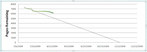
Now I have something Excel is a little better at charting. So long as I set the chart options to "Show empty cells as: Connect data points with line," it ends up looking pretty nice. Using the above test data:

Then I just needed my update macro to insert new rows above the last one to fill in new data whenever I want. My macro looks something like this:

' Find the last cell on the left going down.  This will be the last cell 
' in the "Date" column
Dim left As Range
Set left = Range("A1").End(xlDown)

' Move two columns to the right and select so we have the 3 final cells, 
' including "Date", "Actual remaining", and "Desired remaining"
Dim bottom As Range
Set bottom = Range(left.Cells(1), left.Offset(0, 2))

' Insert a new blank row, and then move up to account for it
bottom.Insert (xlShiftDown)
Set bottom = bottom.Offset(-1)

' We are now sitting on some blank cells very close to the end of the data,
' and are ready to paste in new values for the date and new pages remaining

' (I do this by grabbing some other cells and doing a PasteSpecial into bottom)

Improvement suggestions on that macro are welcome. I just fiddled with it until it worked.

Now I have a pretty chart and I can nerd out all I want with my nerdy books for nerds.